Plotting Swarms with swarm

import numpy as np

N: int = 100 # Number of particles
D: int = 2 # Size of each particle
T: int = 60 # Number of iterations
from typing import Literal

type Swarm =\
        np.ndarray[tuple[Literal['N'],
                         Literal['D']],
                   np.dtype[np.int32]]

type Particle =\
        np.ndarray[tuple[Literal['D']],
                   np.dtype[np.int32]]

Define the Swarm

Define variable \(\mathrm{X}\) that represents the swarm. \(\mathrm{X}\) is a \(N\times D\) matrix, where \(\mathrm{x}_{n,n\in [1,\dots, N]}\) is the \(n^{\mathrm{th}}\) solution and \(x_{n,d}, d\in [1,\dots, D]\) is the \(d^{\mathrm{th}}\) item in that solution. \(\mathrm{Y}\) stores personal bests such that \(\mathrm{Y}_n\) is the personal best of \(\mathrm{X}_n\).

Also, define variable \(X_T\) that stores the history of \(X\). Each \(X_T[t]\) should be \(X\) at time step \(t\). Also define \(Y_T\).

from typing import Callable, Any
import random

# The domain of Any, Any is hard-coded according
#   to D=2.
INITIALISER: Callable[[int, int], float] =\
    lambda _1, _2: np.random.uniform(low = -10, high= -8)

X: Swarm = np.fromfunction(np.vectorize(INITIALISER),
                           shape=(N, D),
                           dtype=float)
Y: Swarm = np.copy(X)

V: Swarm = np.zeros(shape=(N, D),
                    dtype=float)

X_T = []
Y_T = []

Problem and Measure of Success

Define a problem represented by OBJECTIVE. Also define is_better_than, a way to compare two fitnesses.

import ograph.ofunc as ofunc

OBJECTIVE: Callable[[Particle],
                    float] =\
    lambda x: -ofunc.rosenbrock(*x)

is_better_than: Callable[[float, float],
                         bool] =\
    lambda x, y: x > y

# Initialising y_hat to X[0] is arbitrary.
# Would be more "correct" to use Optional.
y_hat: Particle = X[0]
fy_hat: float = OBJECTIVE(y_hat)
y_hat_T: list[Particle] = []
fy_hat_T: list[float] = []

assert X.shape == (N, D)
assert Y.shape == (N, D)
assert V.shape == (N, D)

C_1: float = 1
C_2: float = 1

for _ in range(T):
    # For each iteration:
    # For each particle in swarm:
    for i in range(N):
        fy_i = OBJECTIVE(Y[i])
        fx_i = OBJECTIVE(X[i])

        if is_better_than(fx_i,
                          fy_i):
            Y[i] = X[i]
            fy_i = fx_i

        if is_better_than(fy_i,
                          fy_hat):
            y_hat = Y[i]
            fy_hat = fy_i

    for i in range(N):
        for j in range(len(V[i])):
            r_1j: float = np.random.uniform(0, 1)
            r_2j: float = np.random.uniform(0, 1)
            V[i][j] = V[i][j] +\
                C_1 * r_1j * (Y[i][j]-X[i][j]) +\
                C_2 * r_2j * (y_hat[j]-X[i][j])

        X[i] = X[i] + V[i]


    X_T.append(X.copy())
    Y_T.append(Y.copy())
    y_hat_T.append(y_hat)
    fy_hat_T.append(fy_hat)

Visualisation

Visualise the training process.

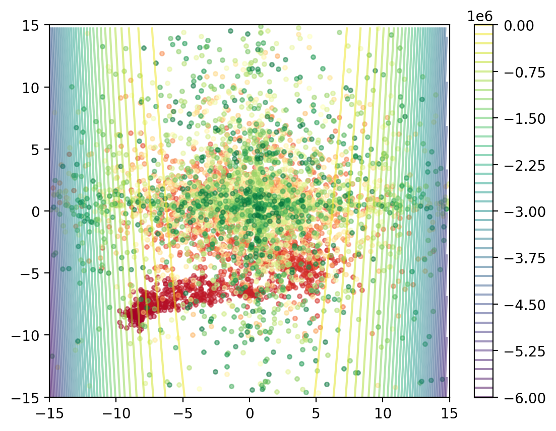
Plot Past Solutions

Plot past values of \(\mathrm{X}\). Recall that \(\mathrm{X}_T[t]\) is \(\mathrm{X}\) at time \(t\).

from ograph.applications.swarm import plot_positions, plot_bests
from ograph.oplot import high_res

high_res()
mort = np.array(X_T)
plot_positions(mort[:,:,:], lambda x, y: OBJECTIVE((x, y)), override_region=((-15, 15), (-15, 15)))

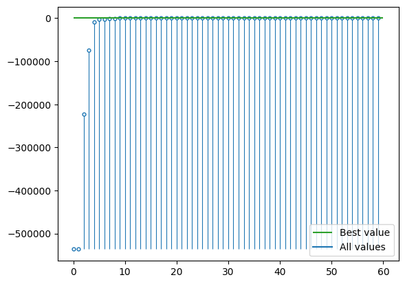
Plot Past Fitnesses

Plot past values of \(f(\hat{y})\).

plot_bests(fy_hat_T)