Collect and Plotting Statistics

This tutorial explains how to collect and plot runtime statistics in two ways:

• The Manual Approach: Collecting fitness values directly from individuals.

• Automating with Watcher: Collecting and reporting fitness values using the evokit.watch module.

import matplotlib.pyplot as plt
import random
random.seed(1)

Construct an Algorithm

For convenience, this tutorial uses a pre-built algorithm that uses the following components.

Component	Choice
Individual	Binary string
Evaluator	OneMax
Selector	Elitist truncation
Variator	Mutation ()

To mimic the size of a practical problem, let’s use the following hyperparameters. All choices are defined as constants in the following cell; please adjust them as you see fit.

Parameter	Choice
Population size	1000
Individual size	10000
Epochs	30

MUTATION_P: float = 0.2
STEP_COUNT: int = 30
POP_SIZE: int = 1000
IND_SIZE: int = 10000

from evokit.evolvables.prefabs import make_onemax

The Manual Approach

Let’s begin with collecting and plotting fitness values by hand. Recall (from the Algorithm tutorial) how everything falls into place:

• The algorithm returned by make_onemax is an instance of HomogenousAlgorithm, which means it has one .population.

• The .population is an instance of Population, which means it is a collection of individuals.

• Each individual is an instance of BitString, a subclass of Individual. All subclasses of Individual inherits the .fitness attribute.

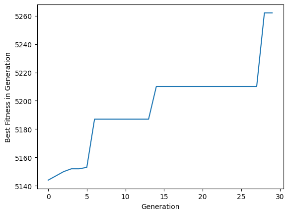
We want to plot the fitness value of the individual with the highest .population. Population.best(...) conveniently returns one such individual; we need only collect and plot its .fitness.

best_fitnesses: list[float] = []

algo = make_onemax(POP_SIZE,
                   IND_SIZE,
                   MUTATION_P,
                   max_parents=0)

for _ in range(STEP_COUNT):
    algo.step()
    best_fitnesses.append(algo.population.best().fitness[0])

plt.plot(range(STEP_COUNT), best_fitnesses)
plt.xlabel("Generation")
plt.ylabel("Best Fitness in Generation")
plt.show()

Automating with Watcher

The evokit.watch module can help collect and report runtime statistics. Compared to the manual, a watch.Watcher can run as soon as events happen, work with a wide range of algorithms, and report data in a easily comparable format.

Components of the module fall into into three categories:

1. The Watcher class, which can both

   1. be called to create simple watchers with custom handlers and

   2. serve as a base class for more complex watchers.

2. The .visualier submodule, which contains tools for plotting collected records.

3. Stock watchers that collect, for example, cpu and memory usage.

This tutorial mainly discusses #1.a and #2.

Inspecting Available Events

The watch module performs its function with the Watcher class. A Watcher can be attached to an Algorithm and respond to certain events fired by the algorithm. Please see the Algorithm tutorial for how an algorithm fires events.

From the user’s perspective, an algorithm can only fire events it declares in .events and .automatic_events. Let’s check these!

algo_2 = make_onemax(POP_SIZE,
                     IND_SIZE,
                     MUTATION_P,
                     max_parents=0)

print(f"events: {algo_2.events};"
      f" automatic events: {algo_2.automatic_events}")

events: ['POST_VARIATION', 'POST_EVALUATION', 'POST_SELECTION']; automatic events: ('POST_STEP',)

These attributes correspond to two sorts of events:

• .events contain manual events. These events can be fired by calling .update (typically from inside .step(...)).

• .automatic_events are fired regardless of how the algorithm is coded. For example, POST_STEP fires after .step(...) is called but before control returns to the caller.

Crafting an Watcher

An watcher must be created with accounting.Watcher. The constructor can take five parameters:

1. A list of events that can trigger collection.

2. A callable handler that collects data from the associated algorithm

3. An optional stride that can space out collections

4. An optional, position-only watch_post_step that decides if the watcher triggers on STEP_END. The last parameter is there for convenience: setting watch_post_step to True has the same effect as adding STEP_END to events.

5. An optional, keyword-only timer. The default time.process_time, while useful for HPC tasks, records the CPU time, which can be much shorter than the actual run time. Let’s use time.perf_counter to drag things out a little.

Let’s declare an Watcher that collects the best fitness from a population only after a step ends. As the type hint shows, the watcher collects…

• … from a SimpleLinearAlgorithm of BitStrings,

• a fitness value of type float.

from evokit.watch import Watcher
from evokit.evolvables.algorithms import SimpleLinearAlgorithm
from evokit.evolvables.bitstring import BitString
import time

fit_acc = Watcher[SimpleLinearAlgorithm[BitString], float](
    events=SimpleLinearAlgorithm.events,
    handler=lambda algo: algo.population.best().fitness[0],
    watch_post_step=True,
    timer=time.process_time)

Registering a Watcher

Once constructed, the watcher can be registered with an algorithm by calling Algorithm.register(...).

Internally, Algorithm.register(...) calls Watcher.subscribe(...) so that the algorithm and the watcher reference each other [^1]. The following figure illustrates this:

algo_2.register(fit_acc)

assert fit_acc in algo_2.watchers
assert algo_2 is fit_acc.subject

Collecting Statistics

Now that everything is in place, let’s run the algorithm and see what happens!

When an event fires in the Algorithm, it calls Algorithm.update which calls Watcher.update for each watcher in the algorithm’s .watchers. Then, the watcher collects statistics from its .subject only if either (a) the event is in its .events or (b) the watcher’s .watch_post_step is True and the event is POST_STEP.

Because POST_STEP triggers only at the end of each .step(...), it’s good practice to fire it at the beginning so that we know how things started. Here goes:

algo_2.update("POST_STEP")
for _ in range(STEP_COUNT):
    algo_2.step()

To inspect what data the watcher has collected, call Watcher.report(...). Note that records collected immediately after POST_VARIATION have value=nan. This is because the variator resets the fitness values of all.

fit_acc.report()[:4]

[WatcherRecord(event='POST_STEP', generation=0, value=nan, time=0.6875),
 WatcherRecord(event='POST_VARIATION', generation=0, value=nan, time=0.6875),
 WatcherRecord(event='POST_EVALUATION', generation=0, value=5180, time=0.6875),
 WatcherRecord(event='POST_SELECTION', generation=0, value=5180, time=0.703125)]

Plotting

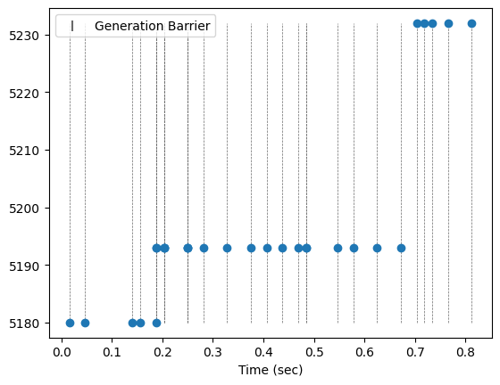
The watch.visual module has tools to plot data from a Watcher. Give it a try! Note that data points are plotted against time. This should make it easier to compare performance.

For simplicity, only end-of-generation fitness values are plotted here. The next section will be much more interesting.

from evokit.watch.visual import plot

plot([x for x in fit_acc.report() if x.event == "POST_STEP"],
     show_generation=True,)

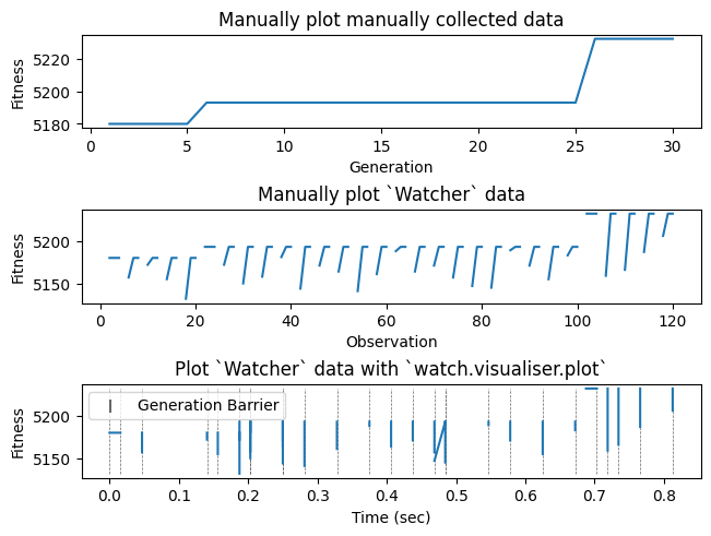
Now the fun begins. Recall that this experiment uses a rather ambitious mutation rate and an elitist selector. The high mutation rate increases the possibility that offspring have a lower best fitness than the parents, but the elitist selector ensures that the best parent is always retained, preventing a generational decline in fitness.

The following cell plots three figures to reflect this:

• The first figure shows what could be collected with the manual approach. As we only have access to the population outside of .step(...), there is not much chance to observe how an elitist selector operates.

• The second figure plots all observed fitnesses. Here, each “hockey stick” shows where the elitist selector updates the population with the best parent.

• The third figure, using watch.visual.plot, plots all data points against time. We see that generations often take different amounts of time, and that the elitist mechanism takes less time to run than what plot 2 suggests,

_, (ax1, ax2, ax3) = plt.subplots(nrows=3,
                                  ncols=1,
                                  layout='constrained')

ax3.set_title("Plot `Watcher` data with `watch.visualiser.plot`")
plot(fit_acc.report(),
     show_generation=True,
     axes=ax3,
     use_line=True)
ax3.set_ylabel("Fitness")


ax2.set_title("Manually plot `Watcher` data")
_data = [x.value for x in fit_acc.report()]
ax2.plot(range(len(_data)), _data)
ax2.set_xlabel("Observation")
ax2.set_ylabel("Fitness")


ax1.set_title("Manually plot manually collected data")
_data = [x.value for x in fit_acc.report() if x.event == "POST_STEP"]
ax1.plot(range(len(_data)), _data)
ax1.set_xlabel("Generation")
ax1.set_ylabel("Fitness")

plt.show()